Scalable Data Science with FHIR

The FHIR standard started as a better way to exchange healthcare data, but it also provides a solid basis for deep analytics and Machine Learning at scale. This post looks at an example from the recent FHIR DevDays conference that does just that. You can also run the interactive FHIR data engineering tutorial used in the conference yourself.

Our first step is to bring FHIR data into a data lake – a computational environment where our analysis can easily and efficiently work through petabytes of data. We’ll look at some patterns for doing so, with concrete examples using the open source Bunsen and Apache Spark projects.

FHIR StructureDefinitions Define the Schema

The schema for every dataset you see here was generated from a FHIR StructureDefinition. There is a big gap between building a FHIR-based schema by hand and generating it directly from the source. Every field in every query here is fully documented as a FHIR resource, making the FHIR documentation itself the primary reference to our datasets. This means the data is well-defined, curated, and familiar to those who have used FHIR.

Data Catalogs over Filesystems

Organizing data in files and directories is convenient, but it becomes unwieldy when working with a large number of complex datasets. Data catalogs can meet this need – and to offer a foundation for further data governance. The Apache Hive metastore is the most common way to catalog data in Hadoop-based environments and has native integration with Spark, so we organize data as one FHIR resource per table. Here’s an example from the tutorial used at FHIR DevDays:

1
2

spark.sql('use tutorial_small')
spark.sql('show tables').toPandas()

Which prints a table like this:

…and so on. This makes it trivial to use intuitive database metaphors like use tutorial_small and select * from condition.

First-class ValueSet Support

FHIR ValueSets – collections of code values for a specific purpose – are essential to querying or working with FHIR data. Therefore they should be a first-class construct in our healthcare data lake. Here’s a look at using some FHIR valuesets in our queries as supported by Bunsen.

1
2
3
4
5
6
7
8

from bunsen.stu3.valuesets import push_valuesets, valueset, isa_loinc, isa_snomed

push_valuesets(spark,
               {'ldl'          : isa_loinc('18262-6'), # Loads LOINC descendants
                'hdl'          : isa_loinc('2085-9'),
                'hypertension' : isa_snomed('38341003'), # Loads SNOMED descendants
                # Loaded from a FHIR ValueSet resource
                'chd'          : valueset('http://engineering.cerner.com/bunsen/example/chd', '201806001')});

Now we can use these valuesets in our SQL queries via the in_valueset user-defined function:

1
2
3
4
5
6
7
8

spark.sql("""
select subject.reference,
       code.coding[0].system system,
       code.coding[0].code code,
       onsetDateTime
from condition
where in_valueset(code, 'chd')
""").limit(10).toPandas()

It’s worth looking at what’s going on here: in a few lines of SQL, we are going from the rich (but somewhat complicated) FHIR Condition data model to a simple table of onset times of Coronary Heart Disease conditions.

FHIR Data in Columnar Storage

Users see a clear catalog of FHIR datasets, but something important is happening behind the scenes. Most data stores or serialization encodings like JSON keep data in a row-wise format. This means all columns from a given record are physically adjacent on disk, like this:

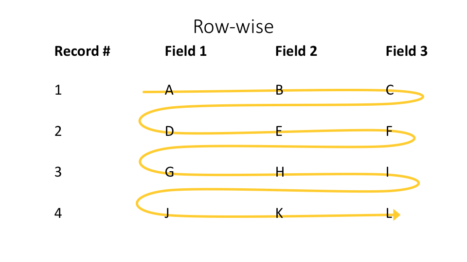
This is a good fit for many workloads, but often not for analysis at scale. For instance, we may want to query the “code” column of several billion observation rows, and retrieve only those in a certain valueset. This is more efficient if columns are grouped together, like this:

This is completely transparent to the user; she simply sees FHIR data from the specification.

So while users see the FHIR data model, it is encoded in a columnar file like Parquet. In such files, all of these “code” columns next to one another, allowing the queries to do tight scans over columns of interest without expensive seeking past unneeded data.

Creating For-Purpose Views

These are the building blocks that simplify otherwise complex analysis. For instance, if we want to identify people with diabetes-related risks, we can create a collection of simple views of the underlying data customized for that purpose. You can see the full example in the Bunsen data engineering tutorial, but we’ll start with a dataframe of people with diabetes-related conditions as defined by a provided ValueSet:

 1
 2
 3
 4
 5
 6
 7
 8
 9
10

diabetes_conditions = spark.sql("""
select id condition_id,
       subject.reference person_ref,
       coding.system,
       coding.code,
       coding.display
from condition
     lateral view explode(code.coding) nested as coding
where in_valueset(code, 'diabetes_risks')
""")

We can inspect and validate this dataframe, and then move onto the next part of our analysis. Let’s say we want to exclude anyone who has had a wellness visit in the last two years from our analysis. We just build a dataframe with them:

1
2
3
4
5
6
7
8

wellness_visits = spark.sql("""
select subject.reference person_ref,
       period.start encounter_start,
       period.end encounter_end
from encounter
where class.code = 'WELLNESS' and
      period.start > '2016'
""")

Now that we’ve loaded and analyzed our dataframes, we can simply exclude those with wellness visits by doing an anti join between them:

1
2
3

diabetes_without_wellness = diabetes_conditions.join(wellness_visits,
                                                     ['person_ref'],
                                                     'left_anti')

The result is a simple table containing the cohort we’re looking for! Check out the complete tutorial notebook for the full story.

Reproducible Results from Immutable Data

Repeatability is an essential property for deep analysis. Re-running the same notebook in the future must load exactly the same data and produce exactly the same results. This gives us the controls needed to build on and iteratively improve previous analysis over time. Fortunately, using immutable data partitions are a common pattern in this type of system. We won’t go into depth here, but will touch on a couple good practices:

• Data is never mutated. Updates coming into our data lake are appended to previous data, and we can reproduce previous results by only working with data that was available at a given processing time.
• If necessary, a policy to archive or remove previous views of data from the data catalog is used to manage size.

Finally, building on such a FHIR-based data lake enables portability. The predictive model or analysis output is fully captured starting with portable data – which means it can be more easily deployed into other systems. FHIR has made great progress in exchanging data in online systems, and we see a lot of promise for data science at scale as well.